PupperPy

Codename: CERBARIS

Our build and extension of the Stanford Pupper Robot. Codename: C.E.R.B.A.R.I.S.

Project maintained by campusrover Hosted on GitHub Pages — Theme by mattgraham

Pupper Vision

For this project, we used the raspberry pi v2 camera to detect and localize our object of interest (tennis ball). At a high level, the vision system works as follows:

Raspberry pi is started
pupper_vision.py is started either as a linux service or by calling it from a higher level python script (such as in run_cerbaris.py). This loads the computer vision model and sets up the picamera.
Use picamera.capture_continuous method to continuously capture frames
Pass each frame through a retrained version of the mobilenet_v2 object detection network
Output top N bounding boxes (according to confidence level assigned by model) with associated class labels
Publish the bounding box info as a list of dictionaries via UDPcomms on port 105

Hardware Interface

Camera

First things first, connect the Raspberry Pi Camera Module to the Pi as in this tutorial. Be sure to make sure the cable is the right way around.

Next, you can enable the camera by using the raspi-config tool. If you do not have the raspi-config tool (e.g. if you are using Ubuntu), you can enable the camera by editing /boot/config.txt (if using raspbian) or /boot/firmware/config.txt (if using Ubuntu). Go to the bottom of the config.txt file and add the lines:

start_x=1
gpu_mem=128

Note, you can increase or decrease gpu_mem to your needs (we currently use 256).

Google Coral Edge TPU USB Accelerator

To accelerate object detection inference onboard the robot, we used the Coral TPU USB accelerator from Google. This plugs into one of the USB 3.0 ports on the raspberry pi 4.

To get started with the USB accelerator, follow the instructions for installing the edgetpu runtime library (replicated here).

echo "deb https://packages.cloud.google.com/apt coral-edgetpu-stable main" | sudo tee /etc/apt/sources.list.d/coral-edgetpu.list
curl https://packages.cloud.google.com/apt/doc/apt-key.gpg | sudo apt-key add -
sudo apt-get update
sudo apt-get install libedgetpu1-std

Tensorflow

The Coral edge TPU is only compatible with Tensorflow Lite and since we only want to do inference with a .tflite model onboard the robot, we will install just the TF Lite interpreter. Make sure to use the .whl for ARM 32 and your corresponding python version (we used python 3.7) e.g.

pip3 install https://github.com/google-coral/pycoral/releases/download/release-frogfish/tflite_runtime-2.5.0-cp37-cp37m-linux_armv7l.whl

ML Models

To perform inference on the TPU, we are able to use the DetectionEngine in the Edge TPU API. This API abstracts away almost all of the tensor manipulation required to do inference. Unfortunately, during the project, this API became deprecated but is still installable via:

sudo apt-get install python3-edgetpu

It has been replaced by the PyCoral API. Which we will endeavour to adapt our code to ASAP.

Given these APIs, all we really need to do is find an object detection model that we can use. Currently, the Edge TPU API only supports SSD (Single-Shot Detection) with a postprocessing operator (such as non-maximum suppression). Additional restrictions on the network operations that are supported on the coral TPU can be found here.

Given the above restrictions, we decided to use a version of MobileNetV2 which is precompiled to be run on the Coral TPU. This model (MobileNetV2 SSD v2 COCO) and a couple other variants are available here. The MobileNet networks, developed by Google, are an attractice option since they utilize a modified convolution operation that requires only ~10% of the computation of a standard convolution operation. This means that they retain most of the accuracy of other vision models but can be run much faster allowing them to be used on mobile and edge devices.

Vision system parameters

There are 2 parameters that you should be aware of when using pupper_vision.py. They are both used in the line:

results = engine.detect_with_image(image,threshold=0.2,keep_aspect_ratio=True,relative_coord=False,top_k=10)

The first parameter is the threshold. For each possible bounding box the network could output, it assigns a ‘confidence’ score. By setting the threshold to some value x, you are specifying that the network will only output bounding boxes (in the results output) with a confidence above the threshold. Therefore, having a low threshold means it is more likely an object will be detected but in practice results in several duplicate boxes around the same object. Lowering the threshold also increases the probability of false positives.
The 2nd parameter is the top_k parameter. This specifies the maximum number of bounding boxes that the model can output for each image. So if top_k=10, the model will output (up to) the 10 bounding boxes with the highest confidence.

Communication with other systems

The pupper_vision.py script is run as a separate process from the control code but must send the bounding box info to be used in the control flow. To accomplish this, the bounding box info for each frame is collected into a list of dictionaries, where each entry in the list contains the height, width, (x,y) location (of top left corner), confidence, and object label of one bounding box. This list of dictionaries is then published via UDPcomms over port 105 (in roman numerals: CV) where the control code can then access the most recent set of bounding boxes.

Transfer Learning

Motivation

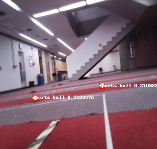
The version of MobileNetV2 mentioned above, was pretrained on the COCO dataset to recognize 90 different object classes. One of these classes is “sports ball” which was close to our desired goal (a tennis ball). We therefore evaluated the performance of this network “out of the box”. We found that while this network was capable of recognizing tennis balls in an image, the tennis ball needed to be fairly close to the robot to be detected and usually had a low associated confidence. This is most likely due to the fact that there were few tennis balls (labeled as sports balls) in the COCO training set. | Undetected | Detected :————————-:|:———————: failure | success

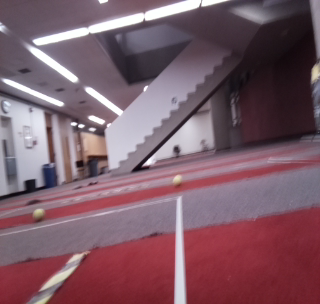We therefore decided to use a transfer learning protocol to retrain the last few layers of the MobileNetV2 on a custom dataset taken from within our robotics lab. We speculated that by retraining specifically on images of tennis balls we would be able to improve the detection range.

Transfer learning is a method for taking a network trained on one dataset, and using the learned features to predict outputs for a new dataset with few examples. The idea is that you remove only the last few layers from the pre-trained network (the layers that essentially map the learned features to output class probabilities) and retrain new output layers on your custom classes. This allows you to reuse the previously learned and hopefully general features in the earlier layers of the network. The retraining process then simply learns a mapping from the pretrained features to your new output classes. This saves lots of training time (since you are training many fewer parameters) and allows you to have fewer examples of your custom classes. In our case, we are hoping to reuse the features learned on the COCO dataset (what this version of mobilenet_v2 was trained on) to learn to detect specifically tennis balls, humans, and chairs (common objects around the robotics lab). The below instructions are meant to be sufficiently general that you could retrain the mobilenet_v2 network on your own custom dataset.

Dataset organization

To collect a custom dataset, we simply placed tennis balls around the robotics lab and continuously captured images using the picamera mounted on the robot. Once the images were acquired, we copied them off of the pi to an Ubuntu laptop (the rest of the retraining procedure all happens off of the pi). The images now need to be labeled by adding bounding boxes around all of the objects we wished to recognize. To do this, we used labelImg which allows you to go through a directory of images and draw boxes around objects in each image. Note that you will need to create a .txt file with all of your desired classes (see the predefined_classes.txt file in the data folder of the labelImg repo for an example). Once you have finished annotating the images, you will have a .xml file for each image with a list of the associated bounding boxes. Go ahead and put all of the image and .xml files into one folder.

We now want to split the annotated dataset into a training set and a test set. For this we’ve written a python script split_data.py which accepts 2 required and 1 optional command line argument.
e.g.

    python3 split_data.py \  
    --data_dir=/path/to/dataset/ \  
    --output_dir=/where/to/store/output/ \  
    --train_frac=0.5   

where train_frac gives the fraction of the total dataset to be used as training data. This will create two directories, train and test, in the output_dir directory.

Once this is done, we need to convert our training and test sets into TFRecord files. To do this we can use the generate_tfrecord.py script in pupperpy/Vision/transfer_learning/. In order to use generate_tfrecord.py you need to install Google’s object detection API. We used the python package installation method:

git clone https://github.com/tensorflow/models.git
cd models/research
protoc object_detection/protos/*.proto --python_out=.
cp object_detection/packages/tf2/setup.py .
python -m pip install --use-feature=2020-resolver .

We will convert the training and test sets separately. For example, for the training set, if all the image and .xml files for the training set are in a directory data/train, run:

python3 generate_tfrecord.py \
--xml_dir=data/train \
--labels_path=/path/to/labels.pbtxt \
--output_path=/path/to/output/tfrecord/train.record \
--image_dir=data/train

If this code runs successfully, there should now be a train.record file in your desired output location. Repeat the same process but for the test set now to create a test.record file.

Lastly, we need to create a label map file called pupper_label_map.pbtxt (see example in the Vision/transfer_learning/learn_custom/custom folder). List all of your desired output classes in this file like this:

item {
  id: 1
  name: 'ball'
}

item {
  id: 2
  name: 'human'
}

item {
  id: 3
  name: 'chair'
}
.
.
.

Retraining the network

Now that we have our train/test.record files, we can move on to actually retraining the network. To do this, we will follow a tutorial on the coral webpage for retraining the last few layers of the mobilenet_v2 model in docker. This tutorial is meant to retrain the network to recognize certain breeds of cats and dogs, but we will utilize the retraining code and just substitute in our own dataset. Note, however that we will need to modify some of the files in the tutorial in order to use our custom dataset.

The first step is to install docker onto your machine.
Follow the instructions in the tutorial for cloning the coral tutorials repo and starting the Docker container. ```shell CORAL_DIR=${HOME}/google-coral && mkdir -p ${CORAL_DIR} cd ${CORAL_DIR} git clone https://github.com/google-coral/tutorials.git cd tutorials/docker/object_detection docker build . -t detect-tutorial-tf1 DETECT_DIR=${PWD}/out && mkdir -p $DETECT_DIR

docker run –name edgetpu-detect
–rm -it –privileged -p 6006:6006
–mount type=bind,src=${DETECT_DIR},dst=/tensorflow/models/research/learn_custom
detect-tutorial-tf1

Note that the line starting with --mount links the directory `DETECT_DIR` in your normal file system to the directory `/tensorflow/models/research/learn_custom` in the docker container's file system. This means that the contents of the `learn_custom` folder in the container are maintained in `DETECT_DIR` even after the docker container is closed (every other newly created folder in the docker container will be erased). This is important to know since if your container closes for some reason before the retraining is finished, any newly created or edited files not in `/tensorflow/models/research/learn_custom` will be lost upon restarting the container.

3. Once you start the docker container, your command prompt should be inside the Docker container at the path `/tensorflow/models/research` and you should see an empty directory titled `learn_custom` inside the research directory. The `learn_pet` directory referenced in the tutorial will not appear since we replaced that with `learn_custom` in the `--mount` flag above. You can create and populate the `learn_pet` directory if you want to run the original tutorial or just to see the file structure if your run the line:
```shell
./prepare_checkpoint_and_dataset.sh --network_type mobilenet_v2_ssd --train_whole_model false

from the original tutorial. This will download the images and annotations, download the model checkpoint, modify the pipeline.config file, and create .record files out of the downloaded dataset. In the steps below we will recreate these steps for our own dataset in the learn_custom directory.

Inside /tensorflow/models/research/learn_custom/ create 4 subdirectories:
```
cd learn_custom
mkdir ckpt models custom train
cd ..
```
Next, you will see a constants.sh file in the research directory. Copy that file to a new file pupper_constants.sh. We need to change the specified paths at the bottom of this file to use our dataset. Change the lines (starting at OBJ_DET_DIR=...) to read the following:
```
OBJ_DET_DIR="$PWD"
LEARN_DIR="${OBJ_DET_DIR}/learn_custom"
DATASET_DIR="${LEARN_DIR}/custom
CKPT_DIR="${LEARN_DIR}/ckpt"
TRAIN_DIR="${LEARN_DIR}/train"
OUTPUT_DIR="${LEARN_DIR}/models"
```
Now save and close this file.

From a terminal outside the docker container, use the docker cp command to copy the train.record, test.record, and pupper_label_map.pbtxt files into the the learn_custom/custom directory in the docker container: e.g.

docker cp /path/to/train.record edgetpu-detect:/tensorflow/models/research/learn_custom/custom
docker cp /path/to/test.record edgetpu-detect:/tensorflow/models/research/learn_custom/custom
docker cp /path/to/pupper_label_map.pbtxt edgetpu-detect:/tensorflow/models/research/learn_custom/custom

Now we need to get the model checkpoint and pipeline files into the learn_custom/ckpt directory. The easiest way to do this is to copy the contents of the Vision/transfer_learning/learn_custom/ckpt directory in the PupperPy repo into the /tensorflow/models/research/learn_custom/ckpt directory in the docker container. e.g.
```
docker cp /path/to/pupperpy/Vision/transfer_learning/learn_custom/ckpt/ edgetpu-detect:/tensorflow/models/research/learn_custom/
```

Alternatively, if you ran the prepare_checkpoint_and_dataset.sh file above, you can copy the contents of the learn_pet/ckpt directory to learn_custom/ckpt

Next, we need to configure the pipeline.config file in learn_custom/ckpt/. If you copied the ckpt directory from the PupperPy repo, you should only need to change the num_classes field below. The critical lines are:
1. (line 19) num_classes: x
  - change whatever x is to the number of classes you want to detect (must agree with the number of classes in you pupper_label_map.pbtxt)
2. (line 27) Make sure this line is type: "ssd_mobilenet_v2"
3. (line 174) This gives the path to the model checkpoint file to use. Make sure it says:
  - fine_tune_checkpoint: "/tensorflow/models/research/learn_custom/ckpt/model.ckpt"
4. (line 194) Gives the path to the .pbtxt label map. Shoud be:
  - label_map_path: "/tensorflow/models/research/learn_custom/custom/pupper_label_map.pbtxt"
5. (line 196) Gives the path to the train.record file. Should be:
  - input_path: "/tensorflow/models/research/learn_custom/custom/train.record"
6. (line 205) Same as line 194, path to .pbtxt label map.
7. (line 209) Path to test.record file. Should be:
  - input_path: "/tensorflow/models/research/learn_custom/custom/test.record"
We are almost ready to begin training. Make sure you are in the /tensorflow/models/research/ directory in the docker container. The last change we need to make is to the retrain_detection_model.sh script. Open this file then go down to the line that says:
```
source "${PWD}/constants.sh"
```
and change this to:
```
source "${PWD}/pupper_constants.sh"
```
Initiate the retraining by running:
```
NUM_TRAINING_STEPS=500 && NUM_EVAL_STEPS=100
./retrain_detection_model.sh \
--num_training_steps ${NUM_TRAINING_STEPS} \
--num_eval_steps ${NUM_EVAL_STEPS}
```
as in the tutorial. This will begin the retraining process using your CPU. As of now we are unsure how to use the code from this tutorial to utilize GPU resources for retraining. The retraining process will likely take several hours depending on how large your custom dataset is.
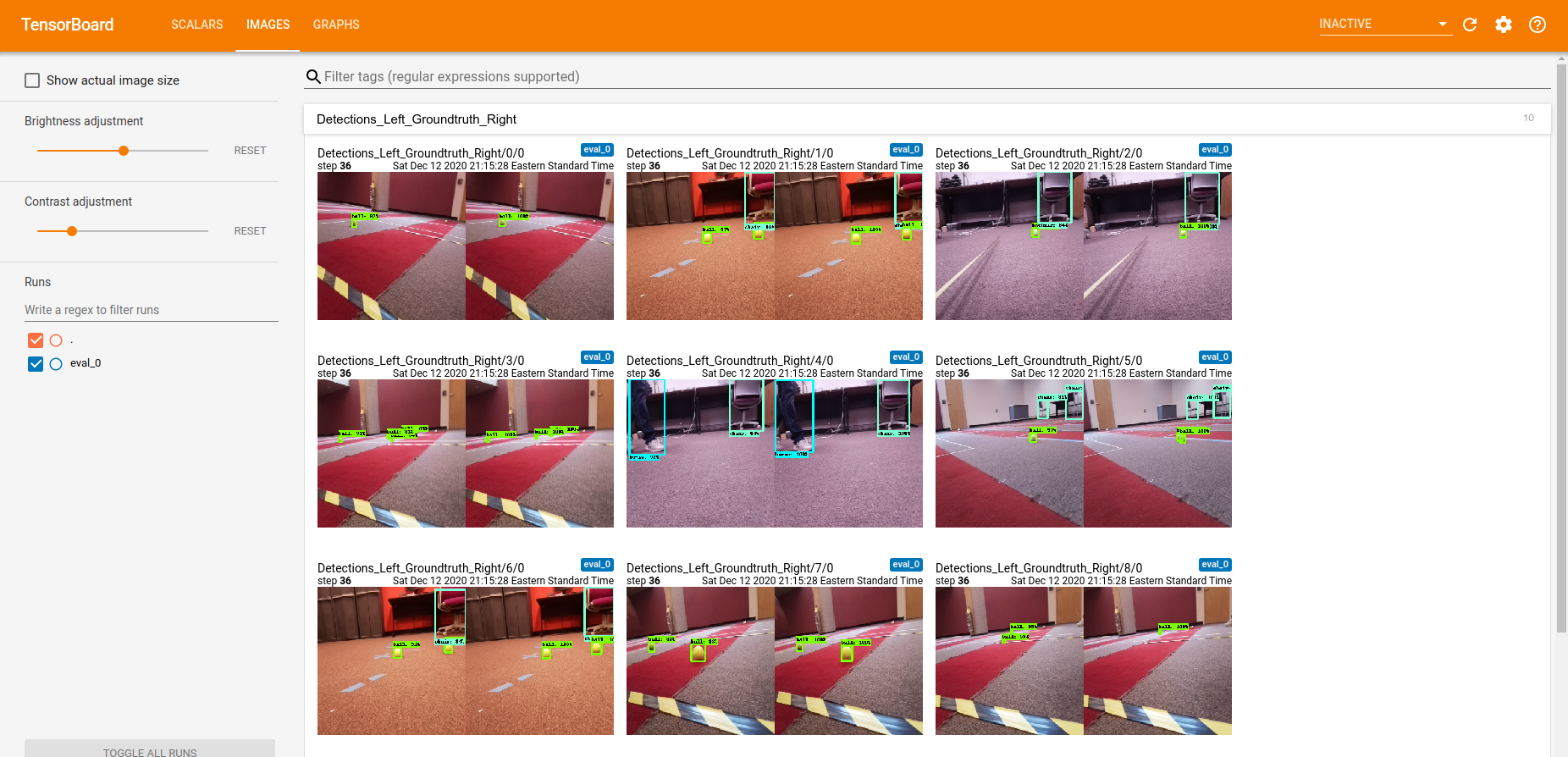
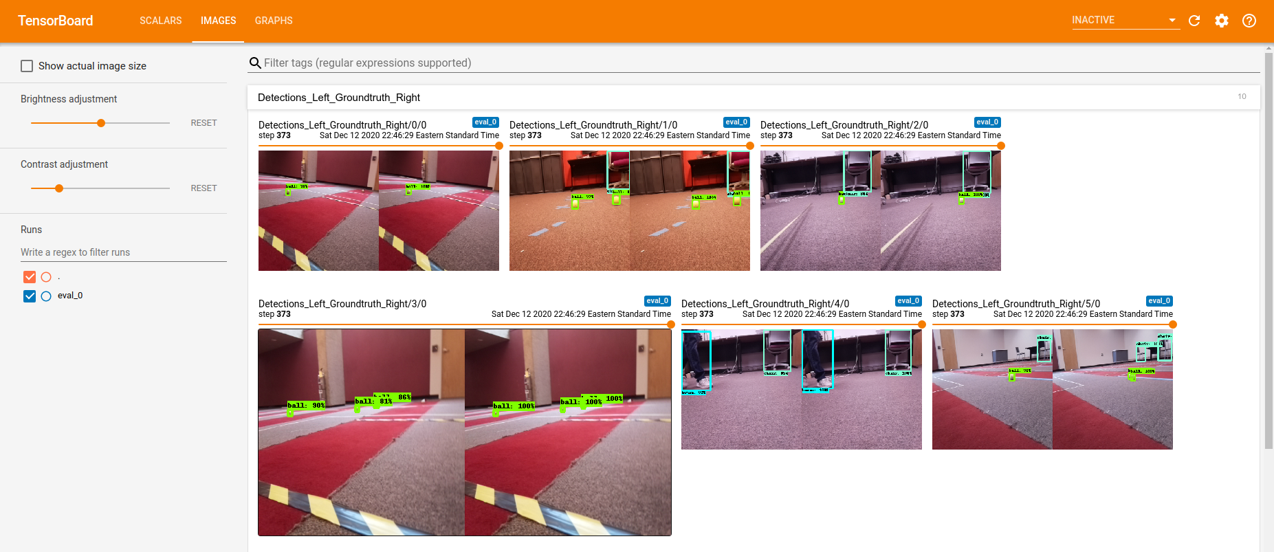
As stated in the tutorial, you can monitor the training progress by starting tensorboard in the docker container. In a new terminal:
```
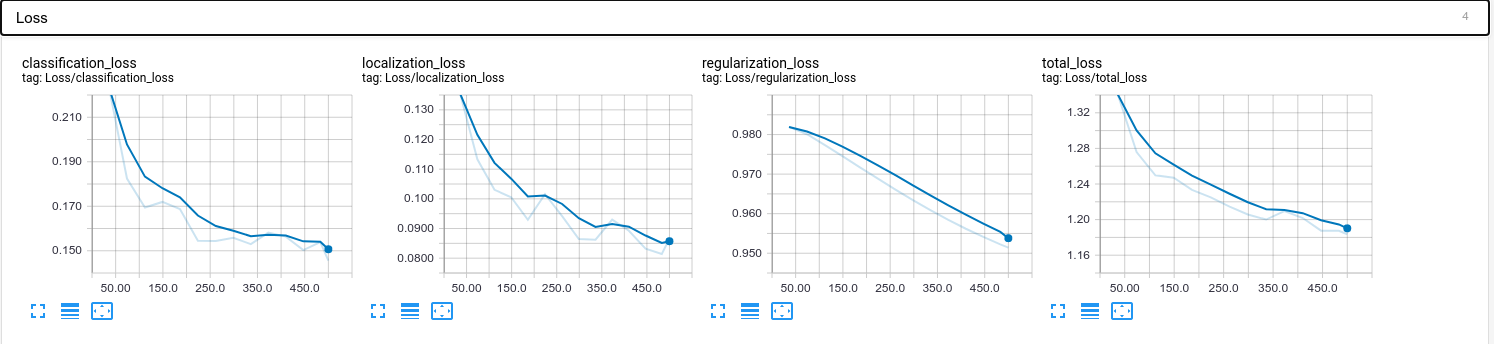
sudo docker exec -it edgetpu-detect /bin/bash
tensorboard --logdir=./learn_custom/train
```
Then you can go to localhost:6006 in your browser and should get a tensorboard panel that will update as training progresses. At first, only the GRAPHS tab will be available, showing you a visualization of the mobilenet network architecture. However, after new checkpoints are saved in learn_custom/train, the SCALARS (showing various training metrics including the loss values) and IMAGES (showing predicted vs ground truth bounding boxes) tabs will appear allowing you to assess the quality of the training.

tensorboard1

tensorboard2

tensorboard3

Compiling the model for the Edge TPU

Now that the network has been retrained, as stated in the tutorial, we need to convert the checkpoint file (found in /tensorflow/models/research/learn_custom/train) to a frozen graph, convert that graph to a TensorFlow Lite flatbuffer file, then compile that model for the Edge TPU. Fortunately the first 2 steps can be done using the convert_checkpoint_to_edgetpu_tflite.sh script in /tensorflow/models/research. However we need to make make one small change first. In convert_checkpoint_to_edgetpu_tflite.sh change the line:

source "${PWD}/constants.sh"

to:

source "${PWD}/pupper_constants.sh"

Now look in the /tensorflow/models/research/learn_custom/train directory and look for the .ckpt file with the highest number (let’s call this number x). This is the most recent checkpoint file (the one from the end of training). We can now convert this checkpoint to a TensorFlow Lite model by calling the following from the /tensorflow/models/research directory:

./convert_checkpoint_to_edgetpu_tflite.sh --checkpoint_num x

where x is the checkpoint number. This will output the TensorFlow Lite model as a file named output_tflite_graph.tflite in the /tensorflow/models/research/learn_custom/models/ directory. Recall that all of the files in the /tensorflow/models/research/learn_custom/ directory in the docker container are also available on your host file system at google-coral/tutorials/docker/object_detection/out if you used the directions above when running the docker container.

Next, follow the instructions in the tutorial (replicated here) to install the Edge TPU Compiler:

curl https://packages.cloud.google.com/apt/doc/apt-key.gpg | sudo apt-key add -
echo "deb https://packages.cloud.google.com/apt coral-edgetpu-stable main" | sudo tee /etc/apt/sources.list.d/coral-edgetpu.list
sudo apt update
sudo apt-get install edgetpu-compiler

Now change to the directory on your host filesystem with the .tflite model (should be ${HOME}/google-coral/tutorials/docker/object_detection/out/models) and run the edgetpu_compiler on the .tflite model.

cd ${HOME}/google-coral/tutorials/docker/object_detection/models
edgetpu_compiler output_tflite_graph.tflite

The compiled file is named output_tflite_graph_edgetpu.tflite and is saved to the current directory. Rename this file to something more descriptive (ours is named ssd_mobilenet_v2_pupper_quant_edgetpu.tflite).

To use the retrained model on the pupper, you will need to add it to the pupperpy/Vision/models directory. In addition, you will need to create a file with the output classes of the model (see pupperpy/Vision/models/pupper_labels.txt for an example) and also put it in the models folder. Lastly, you will need to change the MODEL_PATH and LABEL_PATH lines (lines 23 and 24) in pupper_vision.py to reflect your new model and class files.

Congratulations! The next time you run pupper_vision.py your retrained model will be used. Just be sure to update any exisiting control code to use the class strings from your class file.

Assessment

Below are some examples of the object detection systems ability after the retraining procedure:

tennis_ball_gif

chair_gif

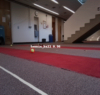
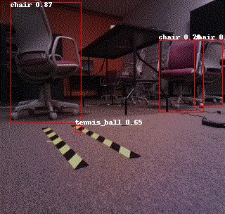
Notice how in the 2nd .gif, the system mistakenly identifies some yellow tape as a tennis ball. This tells us that the network has likely picked up on some simple features of tennis balls (such as that they are yellow) to identify them. This is likely because the training set used to train the network only used images taken from within the robotics lab (where there is not much yellow) and so the network picked out simple features to distinguish them. Additionally, the day the training set was captured, the robot was unable to walk around so the images were taken from only ~12 different angles. This means the system is likely over fit to these angles.

To improve the system it would be beneficial to supplement the existing dataset with images from a diversity of angles (such as from the robot walking around) and settings. However given the very time consuming nature of labeling the images, we have not pursued this.

The dataset we used for retraining can be found here

Future directions

There are 2 additions to the vision system which would be helpful, but that we haven’t had time to implement.

Image stabilization
- While the object detection works fairly well even when the robot is moving, it would likely be improved by stabilizing the images as much as possible. A simple start would be to simply set picamera.video_stabilization = True in pupper_vision.py before the capture_continuous method is run. However, this built in image stabilization only accounts for vertical and horizontal motion.
- An alternative would be to use odometry information from a working IMU (ours is currently not calibrated well enough to use), to rotate/translate captured images. This however will likely reduce the framerate at which images can be processed
Computing distance to target using successive bounding boxes
- One idea we had is that we could use the relative sizes of successive bounding boxes (presumably around the same object) and the velocity of the robot to compute a distance to the target. This, combined with a mapping system, would allow the robot to ‘remember’ where its target is such that it could potentially plan a route there to avoid obstacles if necessary.